TL;DR
Yes, there is a floor on the number of denoising steps, but it is set by the task, not by the model. It scales with how many independent choices the generator must commit to that the conditioning does not already pin down.
Under-determination is the root cause. A prompt like "a giraffe" leaves size, pose, framing and background open. A single network pass must carve Gaussian noise into basins, one per outcome, with sharp boundaries between them. Push-forward theory says that requires a large Lipschitz constant, which is exactly what is hard to learn.
Steps buy sharpness cheaply. Chaining several gentle steps produces a map whose steepness multiplies from step to step. Multi-step sampling lets the model commit coarse-to-fine: the bifurcation ("speciation") happens early, details resolve later. A bigger model raises the per-step budget, but only moves the floor logarithmically.
Well-determined tasks escape the floor. Action prediction conditioned on observations has little residual entropy. FLUX 3 Action ships a 1-step checkpoint that keeps most of the 4-step model's success rate (37.9% vs 41.6% on RoboLab-120): a real but bounded quality cost.
Pretraining conflates two jobs. It teaches what the data looks like (knowledge) and how to denoise any point under an independent noise–data coupling (a harder, high-variance regression). Deployment only needs the first, plus a map from a few noise levels. Reflow and distillation exploit the easier deterministic ODE coupling.
Asymmetric distillation decouples the two. A big teacher and a big critic carry the general-denoising burden at training time; a small, few-step student does the deployed work. Recent DMD results show the critic, not the student, must scale with the teacher.
The implication: few-step generation is the goal, general denoising the scaffolding. Size the student to the task's entropy, not to the pretraining corpus.
1. The cost question: two knobs that are not interchangeable
The inference cost of a diffusion generator comes down to three things: how many times you call the network, how expensive each call is, and a fixed overhead that does not depend on either.
The cost of each call grows with parameter count and with the number of tokens. The fixed overhead covers the text and context encoders, the VAE decoder, and any conditioning on past frames.
That leaves two levers that look symmetric: shrink the network, or cut the number of steps. They are not.
The tempting hope is that capacity can substitute for steps: a model big enough to "see" the whole ODE trajectory could jump to the end in one evaluation. The evidence says capacity helps, but at a poor exchange rate. In Multistep Consistency Models, moving from the small to the large network improves 1-step consistency distillation on ImageNet128 from FID 8.5 to 7.0. Adding a single second step to the small model gets it to 3.1 (Heek et al., 2024). One extra step beats a much larger network.
The rest of this post argues why that exchange rate is structural, where it breaks, and what it means for how we should build fast generators.
2. Under-determination: the giraffe problem
Text-to-image is badly under-determined, and that is the root reason one step is hard. Ask for "a giraffe". The prompt fixes the subject but leaves the rest open: is it close or far, left or right, grazing or running, at dusk or noon, on a savanna or in a zoo? The conditional distribution p(x | prompt) is enormously multimodal, and the generator is given creative license over every free variable.
What a one-step generator has to do
A one-step generator is a deterministic map G from Gaussian noise z to an image. Each z maps to exactly one image, so diversity comes entirely from the noise. That is fine in principle: GANs do it. The difficulty is geometric. G must partition noise space into basins, one per outcome ("giraffe on the left", "giraffe on the right"), and every one of the open choices must be resolved in a single evaluation.
The Gaussian is connected; the set of good images is, to a first approximation, a union of separated modes. A continuous map from a connected set to separated modes must either be very steep at the basin boundaries or put mass in between, where the samples are blends: two half-giraffes, a smeared background. Salmona et al. (NeurIPS 2022) make this precise: for a push-forward model, total variation and KL to a multimodal target are bounded below by a quantity that depends on mode separation and the network's Lipschitz constant. To fit many well-separated modes, the Lipschitz constant must be large. Large Lipschitz constants are what makes training unstable.
What multiple steps buy
Multi-step sampling replaces one steep map with a chain of gentle ones, and steepness compounds along a chain. If each step can stretch distances by at most a factor of 3, two steps can stretch by 9, four steps by 81, eight steps by more than 6,000. The overall map can become almost discontinuous even though no single step is.
That compounding is real, not just an upper limit, whenever successive steps keep amplifying the same direction. That is exactly what happens near a decision: a noise sample leaning slightly toward "giraffe on the left" gets pushed a little further left at every step.
So each step only needs a modest local slope, and the chain still splits noise space cleanly into basins. This is my framing rather than a published theorem. But it is the mechanism Salmona et al. point to when they observe that diffusion models, which stack networks with fresh input at each step, escape the push-forward limit.
It also explains the order in which things happen. Early, high-noise steps commit to the coarse, high-entropy choices (layout, pose, framing). Later steps fill in detail conditioned on those commitments. Each commitment, once made, removes a source of ambiguity for the steps that follow. So "pick a choice and commit to it" is not a figure of speech: it is a sequence of symmetry-breaking events, and the next section shows they can be measured.
3. Bifurcations: why distilled models still need several steps
The commitments described above show up as bifurcations in the sampling dynamics, and they are where one-step students fail.
The physics picture
Raya and Ambrogioni (NeurIPS 2023) study the simplest case: data made of two points, −1 and +1. Early in generation the potential has a single stable fixed point at 0, and every trajectory is symmetric. Past a critical time, that fixed point splits into two stable branches heading to the two data points. A particle gets trapped in one branch, and the authors identify that spontaneous symmetry breaking with the selection of a particular sample. Biroli, Bonnaire, de Bortoli and Mézard (Nature Communications 2024) generalize this to high dimensions: generation passes a speciation transition, where the broad class of the sample is decided, before a later collapse regime where fine detail is fixed. Speciation time can be read off the spectrum of the data's correlation matrix.
At a bifurcation, the dynamics are acutely sensitive to initial conditions. Two noise seeds that differ infinitesimally on either side of the separatrix end in different modes. This is not chaos in the strict dynamical-systems sense, since the flow is smooth and each branch is stable. But it produces the same practical symptom: an exact one-step map must reproduce a discontinuity along every separatrix, for every bifurcation the prompt leaves open.
What Multistep Consistency Models show
Heek, Hoogeboom and Salimans (2024) make the cost visible. Their Figure 1 plots real sampling trajectories of 1-, 2-, 4- and ∞-step consistency models on a two-Gaussian mixture: exactly the toy bifurcation above. They note the 4-step path is smoother than the 1-step path and likely easier to learn. In the text they explain why: the one-step mapping becomes "very sharp and difficult to learn when it jumps between modes" of the target. A precision on attribution: the paper does not use the words bifurcation or chaos. The bifurcation vocabulary comes from the statistical-physics work above; the MCM paper supplies the trajectories and the learning-difficulty argument.
Their remedy is the point. Split the trajectory into a few segments and learn a consistency map per segment. Each segment only spans part of the decision sequence, so each map stays gentle. The numbers bear it out: on ImageNet128 with consistency distillation, the first extra step cuts FID by more than half, while scaling the network barely moves the 1-step result. The table below shows it.
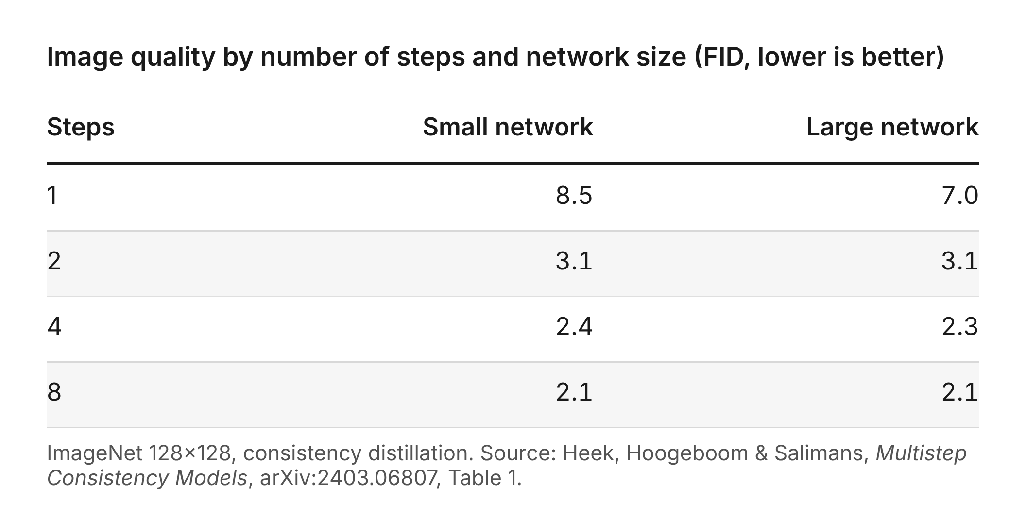
Models trained from scratch show the same pattern more sharply: at 1 step the large network only improves FID from 16.0 to 14.5, while a second step takes the small one to 6.0.
Distillation does not remove this floor; it relocates it. A distilled student still has to reproduce the teacher's separatrices. With N steps, it gets N gentle maps to do it with. With one step, it needs one steep map, and the evidence says that steep map is where the residual FID lives.
4. Well-determined problems: why one step works for actions
If under-determination sets the floor, then a task with little left undetermined should get close to one step. Robot action prediction is such a task, and the evidence fits.
A policy sees camera frames, the robot's own state and an instruction, then outputs the next short chunk of motor commands. Over a horizon of a second or two, the observation pins down most of what should happen next. The conditional distribution of actions is far narrower than that of images given a prompt. There are still a few genuine forks (go around the obstacle on the left or the right), which is why diffusion policies beat plain regression in the first place, but there are few of them.
FLUX 3 Action
Black Forest Labs released FLUX 3 Action on September 23, 2026: a 7B open-weight "world action model" built on the FLUX 3 backbone that jointly denoises future video and action tokens. It ships three inference recipes: a base model with four sampling steps and guidance, a guidance-distilled model, and a step-distilled model that runs in a single step (NYU Shanghai RITS summary). BFL's per-checkpoint success rates on RoboLab-120, averaged over seeds, are:
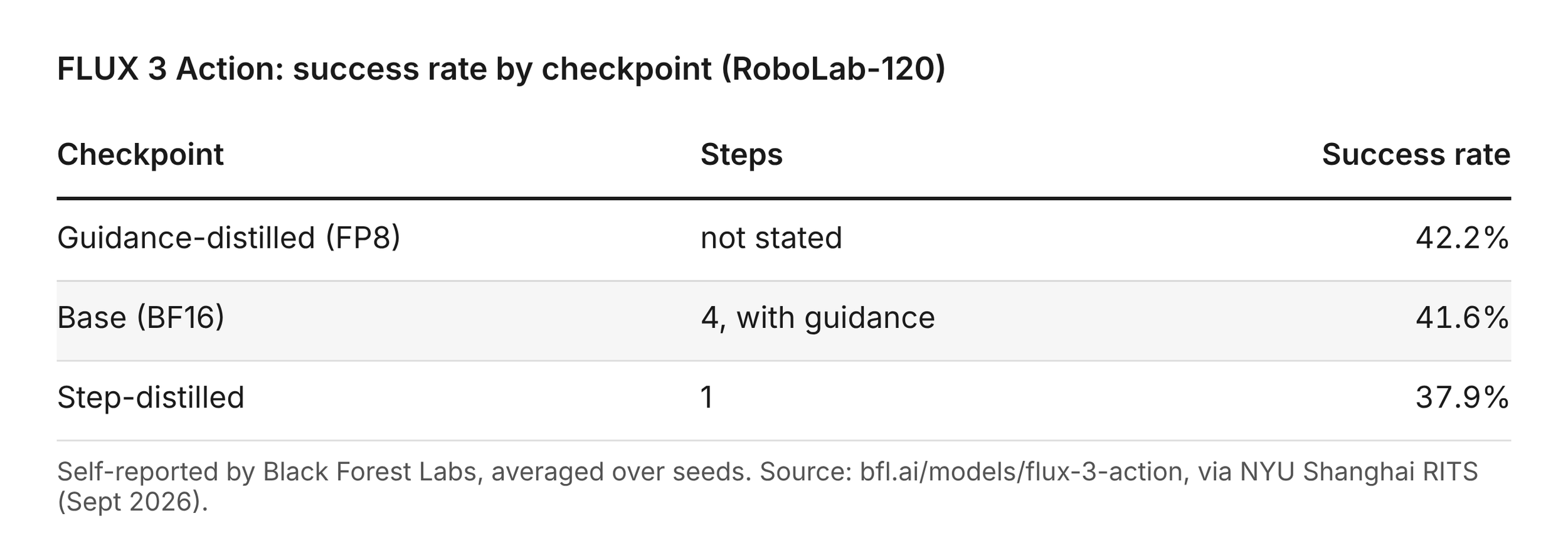
The single-step model keeps about 91% of the base model's success rate. That is the pattern the theory predicts: one step works, and the price is a modest, bounded quality loss, the residue of the few forks the observation does not resolve. Compare that with image generation, where a 1-step student typically loses far more against its multi-step teacher.
The fixed cost shows up
BFL reports 41 ms per inference on a B200 for the BF16 base model and 32 ms for the single-step FP8 variant. Cutting steps by four times saved about a quarter of the latency, and part of that saving comes from the lower precision. Once steps are few, the fixed overhead dominates: encoding context frames and state, and running the model's video branch. That changes where optimization effort should go next, and the cost section below returns to it.
One caveat: these are BFL's self-reported results, and the model predicts video along with actions, so it is not a pure action model. The direction of the result is what matters here.
5. Knowledge versus denoising: two jobs in one set of weights
Diffusion pretraining asks one network to do two different jobs, and only one of them is needed at deployment.
Knowledge. What giraffes look like, how light falls on fur, how a savanna recedes into haze. This is the part that scales with the breadth of the data.
General denoising. Recover a clean estimate from any noisy input at any noise level, where the noise was drawn independently of the image it was added to.
Why the independent coupling is the hard part
In standard training, each image is paired with a fresh random noise sample. Nothing links a particular noise to a particular image. The straight lines between noise and data therefore cross each other everywhere. At a crossing, the same noisy input is consistent with many clean images, so the network can only learn their average, and that average is a blur. The training signal is a noisy regression target whose variance is highest exactly at high noise, where the big decisions are made.
The network must learn this conflicting, averaged field over the entire space, including regions a sampler will never visit. That is a large function to represent, and it is where much of a big model's capacity goes.
Why the ODE coupling is easier
Once a model is trained, running its sampler deterministically defines a new pairing: each noise sample now maps to one specific image. Trajectories of a deterministic flow cannot cross. Every input has exactly one correct target, so the regression has no irreducible noise.
This is what reflow exploits. Liu, Gong and Liu (ICLR 2023) show that retraining on pairs generated by the previous flow gives paths that cross less and less, and that a coupling is fully straight exactly when its paths never intersect. Their first rectified flow already works well with as few as 2 steps; after one round of reflow, it works with a single step.
The limit is instructive. Full straightness needs infinitely many reflow rounds, and in practice some edge cases stay curved: one-step sampling on them produces invalid samples (Zhang et al., 2025). Those edge cases are the separatrices from section 3. The ODE coupling removes the averaging noise, but it cannot remove the decisions. It just hands them, sharp, to whoever must learn the one-step map.
The conflation, stated plainly
A pretrained diffusion model is sized for knowledge plus general denoising under the independent coupling. A deployed few-step generator needs knowledge plus a map from a handful of noise levels under a deterministic coupling. The second job is strictly smaller. There is no reason the deployed network should be as large as the one that learned the field.
6. Asymmetric distillation: let the big networks do the hard job
If the deployed job is smaller than the pretraining job, the obvious move is to keep large networks at training time and ship a small one. Distribution Matching Distillation makes that split natural, and a new paper shows where the capacity has to go.
How DMD divides the work
DMD trains a few-step student by comparing two denoisers on the student's noised outputs: the frozen teacher, which knows what real data looks like, and a "critic" trained online to track what the student currently produces. The gap between them tells the student which way to move. The student never has to match the teacher's trajectories one-to-one, only its distribution (Yin et al., DMD2, 2024). The objective is mode-seeking: it would rather drop a rare mode than smear between two.
Notice which networks carry the general-denoising burden. The teacher and the critic both have to denoise arbitrary noisy inputs at arbitrary noise levels. The student does not; it only has to produce good samples from its few starting points. DMD2 already traced its training instability to a critic that tracked the student's distribution too poorly.
A better critic matters
Wu et al. ("A Better Critic Matters for Distribution Matching Distillation", October 2026), from Adobe and MIT, isolate the critic's role. Across seven SiT sizes on ImageNet, from 33M to 951M parameters, making the teacher bigger while keeping a small critic can hurt the student and even collapse training. Scaling the critic together with the teacher, which they call joint scaling, removes the collapse and lets the student benefit from the bigger teacher. Within each comparison the deployed student keeps the same size and step count (project page).
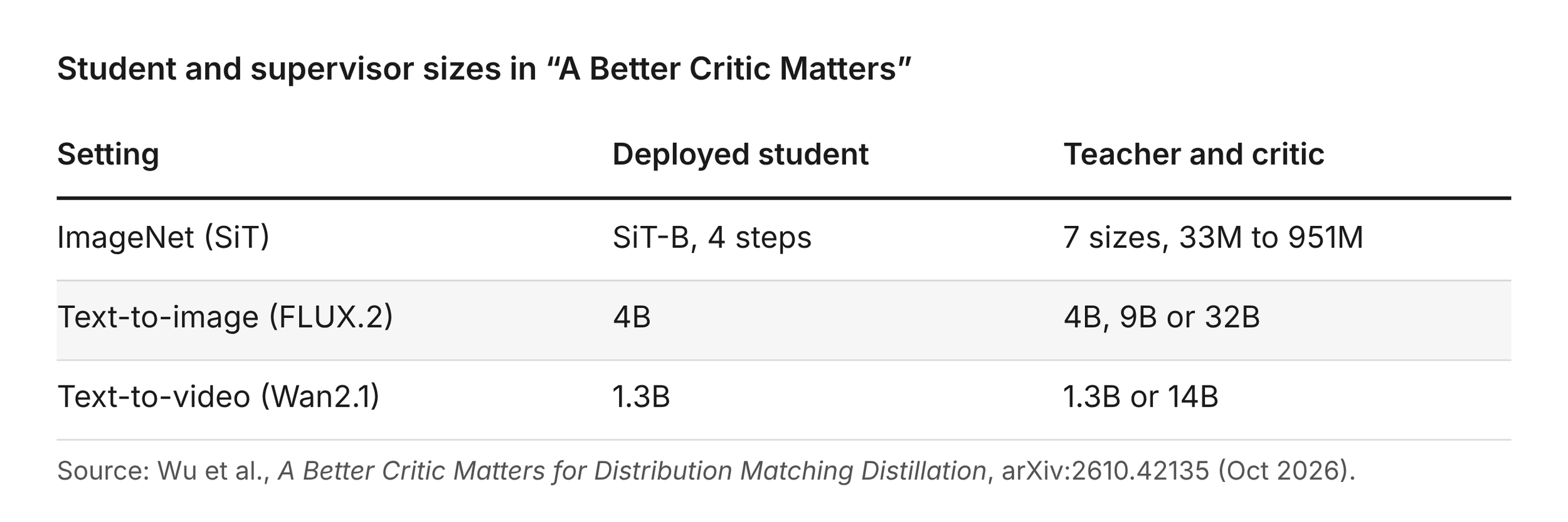
Two results make the point concrete. On ImageNet, a 4-step SiT-B student goes from FID 13.91 to 6.90 with joint scaling plus their second idea. On FLUX.2, pairing a 9B teacher with a 4B critic actually lowers the 4B student's HPSv3 score (10.58 to 10.32); raising the critic to 9B lifts it to 10.92.
The second idea is a step-aware critic (STAC). Instead of modeling one blended distribution over all of the student's steps, the critic is told which step produced a sample and models that step's distribution. That fits the bifurcation picture: the student's intermediate outputs at step 1 and step 3 sit on different sides of the decision sequence, and a critic that averages them gives a muddier signal.
What this says about the thesis
The critic paper is about supervision, not about how small a student can go: it holds the student fixed. But it shows the asymmetry cleanly. Quality is limited by the capacity of the networks that do general denoising at training time, the teacher and the critic. The deployed student can stay small and still improve as those supervisors grow. In other words, the knowledge and the general-denoising burden can live in training-only networks, and the shipped model can be sized to the task.
7. So is there a lower bound?
Yes, but it is a floor on steps set by the task, and a separate floor on cost set by everything around the denoiser. Model size moves neither much.
The floor on steps
The minimum number of steps for high-quality samples is governed by three things.
How much the conditioning leaves open. Every free choice the prompt does not settle is a bifurcation the sampler has to cross. A detailed prompt, a reference image, previous video frames or a robot observation all close choices before sampling starts. Fewer open choices, fewer steps.
How much diversity you insist on keeping. Mode-seeking distillation and classifier-free guidance lower the floor by deleting choices: they shrink the distribution toward its dominant modes. Liu et al. (Decoupled DMD, 2025) go as far as arguing that the guidance-like term is the main engine of DMD distillation, with distribution matching acting as a stabilizing regularizer. The few-step win is partly bought with diversity, and that trade is worth making explicit.
How sharp a map one step can learn stably. A bigger network can learn a somewhat steeper single step, which is why the large model wins at 1 step in the table in section 3. But because sharpness compounds across steps, one extra step is worth far more than a bigger network. Size moves the floor slowly; steps move it fast.
Put together: after you have conditioned as much as you can and given up the diversity you are willing to lose, the remaining number of independent, sharp decisions sets how many steps you need. For a well-conditioned task like control, that can be one. For open-ended text-to-image, today's evidence points to roughly two to four steps before quality plateaus near the teacher.
The floor on cost
Once steps are few, the step count stops being the main cost. FLUX 3 Action shows it: four times fewer steps saved about a quarter of the latency. What remains is the fixed overhead, plus the per-call cost of the student itself. Both of those scale with what the deployed model has to know, which brings the argument back to the student's size, not its step count.
That is the real lower bound on the cost of diffusion-based generation: one or a few calls to a network just large enough for the task's knowledge, plus the encoders and decoders around it. General denoising capacity is not part of that bill.
8. Toward task-shaped few-step generators
We are entering a phase where diffusion generators can run in a few steps and a fraction of the memory, because we size them to the task they actually solve. Few-step generation is the goal. General denoising is the means.
Design principles
Measure the task's open choices before picking a step budget. Ask how much the conditioning leaves undetermined. Next-frame prediction in a world model, action chunks, super-resolution and editing are tightly conditioned; open-ended text-to-image and long-horizon video are not.
Condition harder, not wider. Every bit of context that closes a choice before sampling saves a bifurcation. Autoregressive structure helps here: each new frame is generated given the past ones, so most of the scene is already decided.
Pretrain big, deploy small. Let a large teacher learn the knowledge and the general-denoising field under the independent coupling. Ship a student sized for the knowledge the task needs.
Scale the critic with the teacher. In distribution-matching distillation, an undersized critic wastes a strong teacher and can collapse training. Make the critic step-aware so it does not blur the student's intermediate distributions together.
Spend steps where the decisions are. The bifurcations happen early, at high noise. A schedule that puts its few steps around the speciation regime does more than one spaced evenly.
Decide what diversity is worth. Mode-seeking objectives and guidance lower the step floor by removing modes. For a robot policy that is a feature; for a creative tool it can be a defect. Measure it rather than discovering it in user complaints.
Profile the fixed cost early. Once you reach one to four steps, encoders, decoders and context processing can dominate latency.
Open questions
Can we estimate, from a trained teacher, how many bifurcations a given prompt or observation leaves open, and pick the step count per sample?
How small can the student go? The critic results hold the student fixed; a sweep of student size under a large teacher and critic would settle it.
Can the critic, rather than the student, absorb the knowledge entirely, leaving the student as little more than a decoder for decisions?
What is the right diversity metric for few-step students, so that mode-seeking gains are reported alongside what they cost?
References
Heek, Hoogeboom, Salimans. Multistep Consistency Models. arXiv 2403.06807, 2024.
Salmona, De Bortoli, Delon, Desolneux. Can Push-forward Generative Models Fit Multimodal Distributions?NeurIPS 2022.
Raya, Ambrogioni. Spontaneous Symmetry Breaking in Generative Diffusion Models. NeurIPS 2023.
Biroli, Bonnaire, de Bortoli, Mézard. Dynamical regimes of diffusion models. Nature Communications, 2024.
Liu, Gong, Liu. Flow Straight and Fast: Learning to Generate and Transfer Data with Rectified Flow. ICLR 2023.
Zhang et al. Flow Straighter and Faster: Efficient One-Step Generative Modeling via MeanFlow on Rectified Trajectories. arXiv, 2025.
Yin et al. Improved Distribution Matching Distillation for Fast Image Synthesis (DMD2). NeurIPS 2024.
Wu et al. A Better Critic Matters for Distribution Matching Distillation. arXiv 2610.42135, October 2026. Project page.
Liu et al. Decoupled DMD: CFG Augmentation as the Spear, Distribution Matching as the Shield. arXiv, 2025.
Black Forest Labs. FLUX 3 Action, September 2026; figures as summarized by NYU Shanghai RITS.
Written by Francois Belletti, polished by AI
